Models

Baseline, NLP features, Lexical Diversity

Based on EDA and feature selection, we chose the following baseline features, NLP and Lexical Diversity features. Please refer back to EDA and NLP pages for more details about the selected features. Our approach was to start with the baseline model, then add the NLP features to see if the accuracy improved, and then we added the Lexical Diversity features to improve the model even more. The description below follows a similar trend.

Baseline features	NLP features	Lexical Diversity features
retweet_count	sentiment_negative	LD-log_ttr
favorite_count	sentiment_neutral	LD-uber_index
num_urls	sentiment_positive	LD-yule_s_k
num_mentions	token_count	LD-mtld
num_hashtags	url_token_ratio	LD-hdd
	ratio_neg
	ant
	fear
	joy
	trust
	jaccard

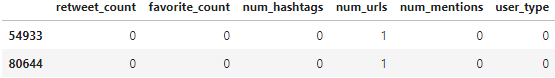
Sample input data

Baseline

Baseline + NLP

Baseline + NLP + Lexical Diversity

KNN

kNN with Baseline features

We have a fairly large number of tweets (over 100K). kNN takes forever to run. We decided drop the kNN from further evaluation.

Xs_train, Xs_test = scale(X_train), scale(X_test)

neighbors, train_scores, cvmeans, cvstds, cv_scores = [], [], [], [], []
for n in range(1,11):
    neighbors.append(n)
    knn = KNeighborsClassifier(n_neighbors = n)
    train_scores.append(knn.fit(X_train, y_train).score(X_train, y_train))
    scores = cross_val_score(estimator=knn,X=Xs_train, y=y_train, cv=5)
    cvmeans.append(scores.mean())
    cvstds.append(scores.std())

Logistic Regression

Logistic Regression (Cross Validated) with Baseline features

Logistic Regression could only achieve a test accuracy of 74%.

model_log_cv_base = LogisticRegressionCV(cv = 5).fit(xtrain_base, ytrain_base)

train_score_logcv_base = model_log_cv_base.score(xtrain_base, ytrain_base)
test_score_logcv_base = model_log_cv_base.score(xtest_base, ytest_base)
print("Log Regression Model Accuracy with Base Features (Train) is ",train_score_logcv_base)
print("Log Regression Model Accuracy with Base Features (Test) is ",test_score_logcv_base)

Log Regression Model Accuracy with Base Features (Train) is 0.7662645518405441 Log Regression Model Accuracy with Base Features (Test) is 0.7640225772312654

LDA/QDA

LDA/QDA with Baseline Features

LDA and QDA performed poorly. They are in the range of 71-75% accuracy.

X_train, y_train = train_base_tweets_df.drop('user_type',axis=1), train_base_tweets_df['user_type']
X_test, y_test = test_base_tweets_df.drop('user_type',axis=1), test_base_tweets_df['user_type']

lda = LinearDiscriminantAnalysis().fit(X_train, y_train)
qda = QuadraticDiscriminantAnalysis().fit(X_train, y_train)

LDA Model Accuracy with Base Features –> LDA score: 0.715240, CV score: 0.716122 QDA Model Accuracy with Base Features –> QDA score: 0.753943, CV score: 0.754397

Decision Tree/RandomForest

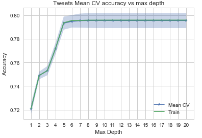
Decision Tree/RandomForest with Baseline Features

The Decision Tree performed well here. After tree depth = 7, the accuracy is not improving. We pick 7 as the optimal tree depth for RandomForest. Given the tree accuracy is fairly constant, the accuracy is ~ 79% for both models.

depths, train_scores, cvmeans, cvstds, cv_scores = [], [], [], [], []
for depth in range(1,21):
    depths.append(depth)
    dt = DecisionTreeClassifier(max_depth=depth)
    train_scores.append(dt.fit(X_train, y_train).score(X_train, y_train))
    scores = cross_val_score(estimator=dt, X=X_train, y=y_train, cv=5)
    cvmeans.append(scores.mean())
    cvstds.append(scores.std())

fitted_rf = RandomForestClassifier(n_estimators=7, max_depth=7).fit(X_train,y_train)
random_forest_train_score = fitted_rf.score(X_train, y_train)
random_forest_test_score = fitted_rf.score(X_test, y_test)

Accuracy with Baseline Features –> 0.79

AdaBoost with Baseline Features

We tuned the parameters of the AdaBoost model and picked a Learning Rate of 0.2, Depth of 2, and 100 estimators to balance accuracy with complexity.

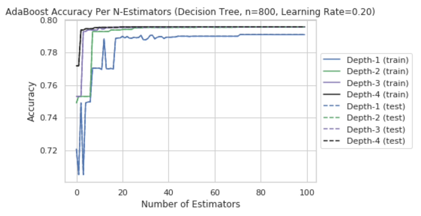
Using those parameters, the AdaBoost model achieved 79% accuracy on the baseline features; only slightly better than Logistic Regression.

```python
#modified from lab 9 notes
def adaboost_build_and_plot(data_tuple, max_depth, n_estimators, learning_rate, makeplot=False, title_or=''):
    X_train = data_tuple[0]
    y_train = data_tuple[1]
    X_test = data_tuple[0]
    y_test = data_tuple[1]

    if len(title_or) > 0:
        title = title_or
    else:
        title = 'AdaBoost Accuracy Per N-Estimators (Decision Tree, Depth-' + str(max_depth) + ', Learning Rate=' + \
                str(learning_rate) + ')'

    skadaboost = AdaBoostClassifier(base_estimator=DecisionTreeClassifier(max_depth=max_depth),
                              n_estimators=n_estimators, learning_rate=learning_rate)
    skadaboost.fit(X_train, y_train)
    print('AdaBoost Accuracy (train)', skadaboost.score(X_train, y_train))
    print('AdaBoost Accuracy (test)', skadaboost.score(X_test, y_test))

    if makeplot == True:

        staged_scores_test = skadaboost.staged_score(X_test, y_test)
        staged_scores_train = skadaboost.staged_score(X_train, y_train)
        plt.figure()
        plt.plot(np.arange(0,n_estimators),list(staged_scores_test), label='AdaBoost Test', linestyle='dashed', color='r')
        plt.plot(np.arange(0,n_estimators),list(staged_scores_train), label='AdaBoost Train', color='b', alpha = 0.6)
        plt.title(title)
        plt.xlabel('Number of Estimators')
        plt.ylabel('Accuracy')
        plt.legend()

t0 = time()
adaboost_build_and_plot(splits['base'], 2, 100, 0.2, makeplot=True)
print("done in %0.3fs." % (time() - t0))

AdaBoost Accuracy (train) 0.7955792191029364
AdaBoost Accuracy (test) 0.7955792191029364
done in 7.316s.

Neural Net with Baseline Features

Neural Network without NLP

In this section we try to use Keras to build a layered Neural Net. We will use a fully-connected network structure with five layers.

Fully connected layers are defined using the Dense class.

We will use the sigmoid activation function on the first layer,softmax activation in the next, rectifier (‘relu‘) activation function on the next two layers and the sigmoid function in the output layer. We use a sigmoid on the output layer to ensure our network output is between 0 and 1 and easy to map to either a probability of class 1 or snap to a hard classification of either class.

We can piece it all together by adding each layer. The first layer has 100 neurons and expects 5 input variables. The second hidden layer has 300 neurons, the third has 100 and the fourth has 50 neurons,respectively.Finally, the output layer has 1 neuron to predict the class (bot or not). We got a mere accuracy of 79%

all_tweets_df_no_nlp = all_tweets[['retweet_count', 'favorite_count', 'num_hashtags', 'num_urls', 'num_mentions','user_type']].sample(frac=.30)
train_base_tweets_df_no_nlp, test_base_tweets_df_no_nlp = train_test_split(all_tweets_df_no_nlp, test_size=0.33, random_state=42, stratify=all_tweets_df_no_nlp['user_type'])

X_train_no_nlp, y_train_no_nlp = train_base_tweets_df_no_nlp.drop('user_type',axis=1), train_base_tweets_df_no_nlp['user_type']
X_test_no_nlp, y_test_no_nlp = test_base_tweets_df_no_nlp.drop('user_type',axis=1), test_base_tweets_df_no_nlp['user_type']

model = Sequential([
    Dense(100, input_shape=(5,), activation='sigmoid'),
    Dense(300, activation='softmax'),
    Dense(100, activation='relu'),
    Dense(50, activation='relu'),
    Dense(1, activation='sigmoid')
])

model.compile(loss='binary_crossentropy', optimizer='adam', metrics=['accuracy'])
model.summary()

_________________________________________________________________
Layer (type)                 Output Shape              Param #   
=================================================================
dense_21 (Dense)             (None, 100)               600       
_________________________________________________________________
dense_22 (Dense)             (None, 300)               30300     
_________________________________________________________________
dense_23 (Dense)             (None, 100)               30100     
_________________________________________________________________
dense_24 (Dense)             (None, 50)                5050      
_________________________________________________________________
dense_25 (Dense)             (None, 1)                 51        
=================================================================
Total params: 66,101
Trainable params: 66,101
Non-trainable params: 0
_________________________________________________________________

history=model.fit(X_train_no_nlp, y_train_no_nlp, epochs=200, batch_size=25, validation_split = .2)

accuracy for Baseline Neural Network: 79.02%

Evaluate Model Accuracy for Extended Features (Baseline + NLP Features + Lexical diversity Features)

Next we used the same model techniques used on the baseline features on the extended features (baseline and NLP features. We observed that accuracy improved for most models with the addition of NLP features.

Input data with Features for NLP and Lexical Diversity

all_tweets_df = all_tweets[['retweet_count', 'favorite_count', 'num_hashtags', 'num_urls', 'num_mentions',
                               'user_type', 'sentiment_negative', 'sentiment_neutral', 'sentiment_positive',
                               'ratio_pos', 'ratio_neg', 'ratio_neu', 'token_count', 'url_token_ratio', 'ant',
                               'disgust', 'fear', 'joy', 'sadness', 'surprise', 'trust','jaccard','LD-uber_index','LD-yule_s_k','LD-mtld','LD-hdd']]

Logistic Regression (Cross Validated) with Extended Features

Logistic Regression (Cross Validated) with NLP features

We were able to bring the accuracy a little bit up to 82.47% after adding the NLP features

model_log_cv = LogisticRegressionCV(cv = 5).fit(xtrain_nlp, ytrain_nlp)

train_score_logcv_nlp = model_log_cv.score(xtrain_nlp, ytrain_nlp)
test_score_logcv_nlp = model_log_cv.score(xtest_nlp, ytest_nlp)
print("Log Regression Model Accuracy with NLP (Train) is ",train_score_logcv_nlp)
print("Log Regression Model Accuracy with NLP (Test) is ",test_score_logcv_nlp)

Log Regression Model Accuracy with NLP (Train) is 0.8250179958795641 Log Regression Model Accuracy with NLP (Test) is 0.824749281862621

Logistic Regression (Cross Validated) with NLP and Lexical Diversity features

Next we added Lexical Diversity features to the mix and it went very slightly higher to 82.7%

model_log_cv_base = LogisticRegressionCV(cv = 5).fit(xtrain_base, ytrain_base)

train_score_logcv_base = model_log_cv_base.score(xtrain_base, ytrain_base)
test_score_logcv_base = model_log_cv_base.score(xtest_base, ytest_base)
print("Log Regression Model Accuracy with Base Features (Train) is ",train_score_logcv_base)
print("Log Regression Model Accuracy with Base Features (Test) is ",test_score_logcv_base)

Log Regression Model Accuracy with Base Features (Train) is  0.8267182962245886
Log Regression Model Accuracy with Base Features (Test) is  0.8271430731240236

LDA/QDA with Extended Features

Even with NLP features added, the accuracy of the LDA is 81% and 75% for QDA. We decided to drop these models from further evaluation and concentrated on the models that are doing really well.

LDA/QDA with NLP Features added

Next we added the NLP features to see if there was improvement.We got an accuracy of around 81%

lda = LinearDiscriminantAnalysis().fit(X_train, y_train)
qda = QuadraticDiscriminantAnalysis().fit(X_train, y_train)
print("LDA score: %f, CV score: %f" % (accuracy_score(y_test, lda.predict(X_test)), cross_val_score(estimator=lda, X=X_test, y=y_test, cv=5).mean()))
print("QDA score: %f, CV score: %f" % (accuracy_score(y_test, qda.predict(X_test)), cross_val_score(estimator=qda, X=X_test, y=y_test, cv=5).mean()))

LDA Model Accuracy with Base Features –> LDA score: 0.810487, CV score: 0.810311 QDA Model Accuracy with Base Features –> QDA score: 0.759008, CV score: 0.763846

LDA/QDA with Lexical Diversity Features added

Again with Lexical Diversity Features added, we get a very slight improvement of 81.2%

lda = LinearDiscriminantAnalysis().fit(X_train, y_train)
qda = QuadraticDiscriminantAnalysis().fit(X_train, y_train)
print("LDA score: %f, CV score: %f" % (accuracy_score(y_test, lda.predict(X_test)), cross_val_score(estimator=lda, X=X_test, y=y_test, cv=5).mean()))
print("QDA score: %f, CV score: %f" % (accuracy_score(y_test, qda.predict(X_test)), cross_val_score(estimator=qda, X=X_test, y=y_test, cv=5).mean()))

LDA Model Accuracy with Base Features –> LDA score: 0.811369, CV score: 0.811873 QDA Model Accuracy with Base Features –> QDA score: 0.774228, CV score: 0.735321

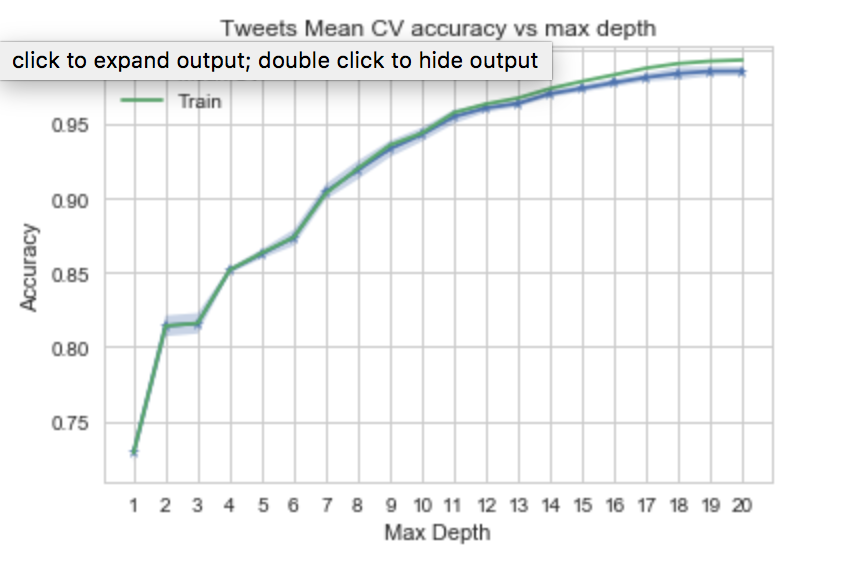
Decision Tree/RandomForest with Extended Features

With the addition of NLP features, the DecisionTreeClassifier accuracy improved dramatically. The graph shows over fitting starting at depth = 13. We will select depth = 12 as the optimal depth for RandomForest. The RandomForestClassifier accuracy is lower than decision tree because it is an average result over multiple estimators (DecisionTree).

Decision Tree/RandomForest with NLP Features

The Decision Tree performed well here. After tree depth = 12, the accuracy did not improve, so we chose 12 as the optimal tree depth. The accuracy shot up to about 96%

depths, train_scores, cvmeans, cvstds, cv_scores = [], [], [], [], []
for depth in range(1,21):
    depths.append(depth)
    dt = DecisionTreeClassifier(max_depth=depth)
    train_scores.append(dt.fit(X_train, y_train).score(X_train, y_train))
    scores = cross_val_score(estimator=dt, X=X_train, y=y_train, cv=5)
    cvmeans.append(scores.mean())
    cvstds.append(scores.std())

#Choosing the best depth
idx = depths.index(12)
print("Accuracy: Mean={:.3f}, +/- 2 SD: [{:.3f} -- {:.3f}]".format(
    cvmeans[idx], cvmeans[idx] - 2*cvstds[idx], cvmeans[idx] + 2*cvstds[idx]))

Accuracy with NLP Features –> Mean=0.961, +/- 2 SD: [0.958 – 0.964]

 fitted_rf = RandomForestClassifier(n_estimators=10, max_depth=12).fit(X_train,y_train)
 random_forest_train_score = fitted_rf.score(X_train, y_train)
 random_forest_test_score = fitted_rf.score(X_test, y_test)
 print(f"The Random Forest scored {random_forest_train_score:.3f} on the training set.")
 print(f"The Random Forest scored {random_forest_test_score:.3f} on the test set.")

The Random Forest scored 0.928 on the training set. The Random Forest scored 0.923 on the test set.

Decision Tree/RandomForest with Lexical Diversity Features

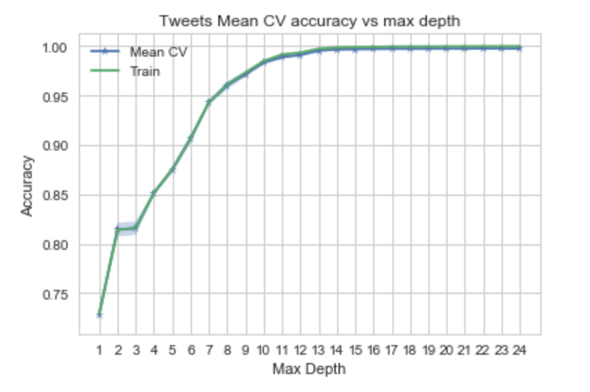
The Decision Tree performed well here. After tree depth = 12, the accuracy is not improving. We picked 12 as the optimal tree depth. The accuracy shot up to about 99%.

#Perform 5-fold cross validation and store results
depths, train_scores, cvmeans, cvstds, cv_scores = [], [], [], [], []
for depth in range(1,25):
    depths.append(depth)
    dt = DecisionTreeClassifier(max_depth=depth)
    train_scores.append(dt.fit(X_train, y_train).score(X_train, y_train))
    scores = cross_val_score(estimator=dt, X=X_train, y=y_train, cv=5)
    cvmeans.append(scores.mean())
    cvstds.append(scores.std())
    ```

![Decision Tree with NLP features](/cs109a/image/DS_NLP_LD.png)

```python
#Choosing the best depth
idx = depths.index(12)
print("Accuracy: Mean={:.3f}, +/- 2 SD: [{:.3f} -- {:.3f}]".format(
    cvmeans[idx], cvmeans[idx] - 2*cvstds[idx], cvmeans[idx] + 2*cvstds[idx]))

Accuracy with LD Features –> Accuracy: Mean=0.991, +/- 2 SD: [0.990 – 0.993]

#Evaluate performance on Test Set
best_cv_depth = 12
fitted_tree = DecisionTreeClassifier(max_depth=best_cv_depth).fit(X_train, y_train)
best_cv_tree_train_score = fitted_tree.score(X_train, y_train)
best_cv_tree_test_score = fitted_tree.score(X_test, y_test)
print(f"The tree of depth {best_cv_depth} achieved an Accuracy of {best_cv_tree_test_score:.3f} on the test set.")

The tree of depth 12 achieved an Accuracy of 0.993 on the test set.

 #Fit a Random Forest model
fitted_rf = RandomForestClassifier(n_estimators=7, max_depth=13).fit(X_train,y_train)
random_forest_train_score = fitted_rf.score(X_train, y_train)
random_forest_test_score = fitted_rf.score(X_test, y_test)
print(f"The Random Forest scored {random_forest_train_score:.3f} on the training set.")
print(f"The Random Forest scored {random_forest_test_score:.3f} on the test set.")

The Random Forest scored 0.985 on the training set. The Random Forest scored 0.982 on the test set.

AdaBoost Accuracy with Extended features

AdaBoost Accuracy with NLP Features added

As seen below, the addition of the NLP features improved the accuracy of the model by nearly 20%.

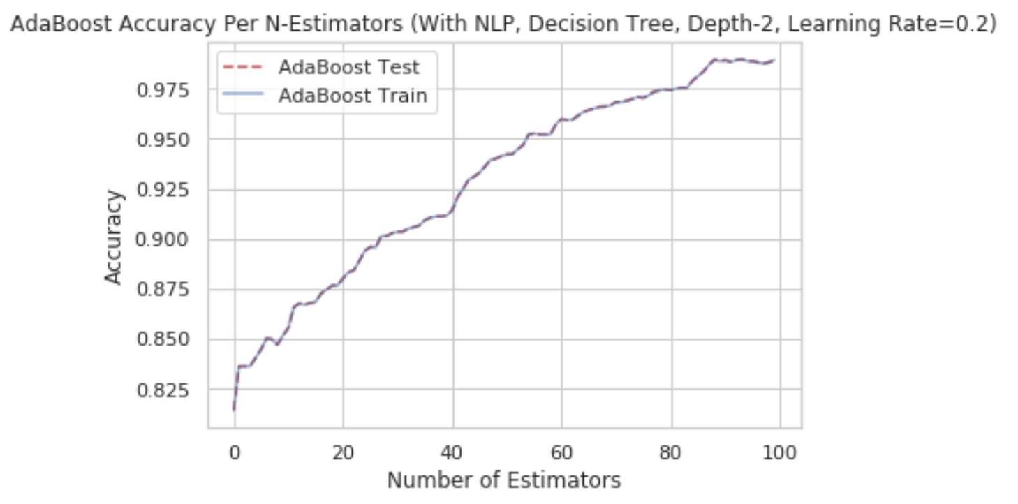
adaboost_build_and_plot(splits['nlp'],2,100,0.2, makeplot=True, title_or="AdaBoost Accuracy Per N-Estimators (With NLP, Decision Tree, Depth-2, Learning Rate=0.2)")
print("done in %0.3fs." % (time() - t0))

AdaBoost Accuracy (train) 0.9893017598729119
AdaBoost Accuracy (test) 0.9893017598729119
done in 11.563s.

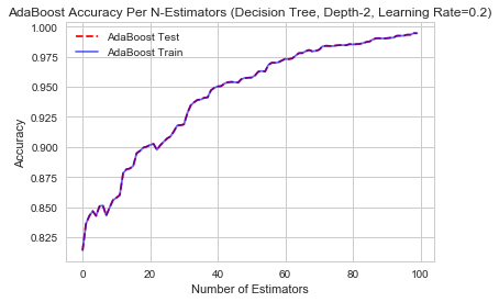
AdaBoost Accuracy with Lexical Diversity Features added

On Including Lexical Diversity for ADABoost we saw an impressive jump to 99.44%

#adaboost_build_and_plot(data_tuple, max_depth, n_estimators, makeplot=False, iterate=False)
t0 = time()
adaboost_build_and_plot(splits['nlp'],2,100,0.2, makeplot=True)
print("done in %0.3fs." % (time() - t0))

AdaBoost Accuracy (train) 0.9944026609079852
AdaBoost Accuracy (test) 0.9944026609079852
done in 21.969s.

Neural Network Accuracy with Extended features

Neural Network Accuracy with NLP and Lexical Diversity Features added

model_nlp = Sequential([
    Dense(100, input_shape=(25,), activation='sigmoid'),
    Dense(300, activation='softmax'),
    Dense(100, activation='relu'),
    Dense(50, activation='relu'),
    Dense(1, activation='sigmoid')
])

model_nlp.compile(loss='binary_crossentropy', optimizer='adam', metrics=['accuracy'])

  history = model_nlp.fit(X_train, y_train, epochs=100, batch_size=32, validation_split = .2)

  NN_testScore_ld=model_nlp.evaluate(X_test, y_test)
  print("\n%s: %.2f%%" % (model_nlp.metrics_names[1], NN_testScore_ld[1]*100))

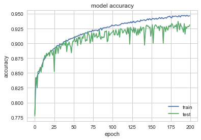
Accuracy with Neural Network and adding NLP and Lexical Diversity features: 93%